Capstone Project: Route Planner
Turn the graph toolkit from this course into a real product.
Introduction
Welcome to the capstone! Every lesson so far taught one tool. This project is where they come together. You'll build a route planner for a small map of towns and roads, and answer four very different questions about it, each one a different algorithm from the course: is the network connected (BFS), what is the fewest-stops route (BFS shortest path), what is the fastest route (Dijkstra + a heap), and which roads are cheapest to build to connect every town (a minimum spanning tree). The real skill this project trains is not any single algorithm, it is recognizing which tool a problem is asking for, then reaching for it with confidence.
Project Purpose
The goal is a small command-line route planner that loads a weighted map and answers routing questions about it. Here is the map we will work with: six towns A to F, connected by roads whose weights are travel times in minutes.
The Map: 6 Towns, Roads Labeled in Minutes
Figure 1: The road network. Note A connects to F directly (14 min), but A-C-F is only 9 + 2 = 11.
Why This Project Matters
A map is just a weighted graph, and "what is the best route" is one of the most common real questions in software. Building this planner exercises the full graph toolkit:
- Graph modeling, representing a real network as a weighted adjacency list (Lesson 13)
- Traversal, using breadth-first search to answer reachability and fewest-stops questions (Lesson 13)
- Shortest paths, using Dijkstra's algorithm and a priority queue for fastest routes (Lessons 20 and 9)
- Minimum spanning trees, using Kruskal's algorithm and union-find for the cheapest network (Lesson 20)
- Complexity reasoning, justifying each choice by its running time (Lesson 1)
The same code powers GPS navigation, network routing, logistics, and game pathfinding. A map of towns is the friendliest way to see it, but the algorithms are exactly the ones production systems use.
First Steps
Step 1: Create Your Project Folder
Start by creating a dedicated folder for the capstone:
mkdir route-plannercd route-plannerStep 2: Create the Virtual Environment
Set up an isolated Python environment:
python3 -m venv .venvsource .venv/bin/activateStep 3: No Dependencies Needed
There is no requirements.txt for this project. Everything we need ships with Python's standard library:
heapq
The min-heap from Lesson 9, used as Dijkstra's priority queue to always expand the closest town next.
collections.deque
The O(1) queue from Lesson 4, used as the BFS frontier for reachability and fewest-stops routing.
Project Structure
We will separate the map from the algorithms that run on it, so each file has one clear job. The layout is flat: three modules plus an empty __init__.py, all in the project folder:
touch graph.py planner.py main.py __init__.pygraph.py
The Graph class: the map itself, stored as a weighted adjacency list.
planner.py
The RoutePlanner class: one method per routing question, each a course algorithm.
main.py
Builds the example map and runs every feature, printing the results.
Implementing graph.py
The map is a weighted, undirected graph. We store it as an adjacency list: a dict mapping each town to a list of (neighbor, minutes) pairs.
graph.py - Complete Implementation
class Graph:
    """An undirected, weighted map: towns connected by roads (weight = minutes)."""

    def __init__(self) -> None:
        self._adj: dict[str, list[tuple[str, int]]] = {}

    def add_town(self, name: str) -> None:
        self._adj.setdefault(name, [])

    def add_road(self, a: str, b: str, minutes: int) -> None:
        self.add_town(a)
        self.add_town(b)
        self._adj[a].append((b, minutes))   # roads run both ways
        self._adj[b].append((a, minutes))

    def towns(self) -> list[str]:
        return list(self._adj)

    def neighbors(self, town: str) -> list[tuple[str, int]]:
        return self._adj[town]
What's Happening Here?
- Adjacency list, not a matrix, real road maps are sparse (each town touches only a few others), so a list of neighbors uses O(V + E) memory instead of a matrix's O(V²) (Lesson 13).
- Roads run both ways,
add_roadappends the edge to both towns, which is what makes the graph undirected. - setdefault, adding a town is idempotent, so calling
add_roadfor a brand-new town just works without a separate registration step.
Implementing planner.py
This is the heart of the project. Each method answers one routing question by picking the algorithm that fits it. Notice that fewest_stops and fastest_routeboth find a "shortest" path, but they mean different things, and that is the whole point.
planner.py - Complete Implementation
import heapq
from collections import deque

from graph import Graph


class RoutePlanner:
    """Answers routing questions about a Graph, each with the right algorithm."""

    def __init__(self, graph: Graph) -> None:
        self.graph = graph

    def reachable_from(self, start: str) -> set[str]:
        # BFS flood fill (Lesson 13): every town you can get to from "start"
        seen = {start}
        queue = deque([start])
        while queue:
            town = queue.popleft()
            for neighbor, _ in self.graph.neighbors(town):
                if neighbor not in seen:
                    seen.add(neighbor)
                    queue.append(neighbor)
        return seen

    def is_connected(self) -> bool:
        towns = self.graph.towns()
        return len(self.reachable_from(towns[0])) == len(towns)

    def fewest_stops(self, start: str, goal: str) -> list[str] | None:
        # BFS shortest path (Lesson 13): fewest legs, ignoring travel time
        parent = {start: None}
        queue = deque([start])
        while queue:
            town = queue.popleft()
            if town == goal:
                break
            for neighbor, _ in self.graph.neighbors(town):
                if neighbor not in parent:
                    parent[neighbor] = town
                    queue.append(neighbor)
        return self._rebuild_path(parent, goal)

    def fastest_route(self, start: str, goal: str) -> tuple[list[str] | None, float]:
        # Dijkstra (Lesson 20) with a min-heap (Lesson 9): fewest minutes
        distance = {town: float("inf") for town in self.graph.towns()}
        distance[start] = 0
        parent = {start: None}
        visited: set[str] = set()
        heap = [(0, start)]
        while heap:
            dist, town = heapq.heappop(heap)
            if town in visited:
                continue
            visited.add(town)
            for neighbor, minutes in self.graph.neighbors(town):
                if dist + minutes < distance[neighbor]:
                    distance[neighbor] = dist + minutes
                    parent[neighbor] = town
                    heapq.heappush(heap, (distance[neighbor], neighbor))
        return self._rebuild_path(parent, goal), distance[goal]

    def cheapest_network(self) -> tuple[list[tuple[str, str, int]], int]:
        # Kruskal's MST + union-find (Lesson 20): min roads to connect every town
        root = {town: town for town in self.graph.towns()}

        def find(x: str) -> str:
            while root[x] != x:
                root[x] = root[root[x]]   # path compression
                x = root[x]
            return x

        def union(a: str, b: str) -> bool:
            ra, rb = find(a), find(b)
            if ra == rb:
                return False              # already connected: this edge would form a cycle
            root[rb] = ra
            return True

        edges = set()
        for town in self.graph.towns():
            for neighbor, minutes in self.graph.neighbors(town):
                a, b = sorted((town, neighbor))
                edges.add((minutes, a, b))

        chosen: list[tuple[str, str, int]] = []
        total = 0
        for minutes, a, b in sorted(edges):   # cheapest road first
            if union(a, b):
                chosen.append((a, b, minutes))
                total += minutes
        return chosen, total

    @staticmethod
    def _rebuild_path(parent: dict[str, str | None], goal: str) -> list[str] | None:
        if goal not in parent:
            return None                   # goal was never reached
        path = []
        current = goal
        while current is not None:
            path.append(current)
            current = parent[current]
        return path[::-1]
What's Happening Here?
- reachable_from / is_connected, a plain BFS flood fill (Lesson 13). Start a queue at one town and visit outward; if you reach every town, the network is connected. O(V + E).
- fewest_stops, BFS shortest path (Lesson 13). BFS visits towns in order of distance in hops, so the first time it reaches the goal is via the fewest legs. The
parentdict remembers how we got to each town, so we can rebuild the route. - fastest_route, Dijkstra's algorithm (Lesson 20) driven by a min-heap(Lesson 9). It always expands the closest unvisited town, relaxes its roads, and records a
parentfor path rebuilding. O((V + E) log V). - cheapest_network, Kruskal's MST with union-find (Lesson 20). Sort every road cheapest-first and add it only if its two towns are not already connected (union-find's O(nearly 1) check), which avoids cycles. O(E log E).
- _rebuild_path, the shared trick behind both routing methods: follow the
parentpointers backward from the goal, then reverse. This is why we get the actual route, not just its length.
Implementing main.py
Finally, wire it together: build the example map from Figure 1, then run every feature and print the results.
main.py - Complete Implementation
from graph import Graph
from planner import RoutePlanner


def build_map() -> Graph:
    graph = Graph()
    roads = [
        ("A", "B", 7), ("A", "C", 9), ("A", "F", 14), ("B", "C", 10),
        ("B", "D", 15), ("C", "D", 11), ("C", "F", 2), ("D", "E", 6), ("E", "F", 9),
    ]
    for a, b, minutes in roads:
        graph.add_road(a, b, minutes)
    return graph


def main() -> None:
    planner = RoutePlanner(build_map())

    print("== ByteCode Route Planner ==")
    print("Towns:", ", ".join(sorted(planner.graph.towns())))
    print()

    reachable = planner.reachable_from("A")
    print("Reachable from A:", ", ".join(sorted(reachable)))
    print("Network connected:", planner.is_connected())
    print()

    stops = planner.fewest_stops("A", "F")
    legs = len(stops) - 1
    print(f"Fewest stops A -> F: {' -> '.join(stops)}  ({legs} leg{'s' if legs != 1 else ''})")

    route, minutes = planner.fastest_route("A", "F")
    print(f"Fastest route A -> F: {' -> '.join(route)}  ({minutes} min)")
    print("   the 2-leg detour beats the direct 14-min road!")
    print()

    network, cost = planner.cheapest_network()
    print("Cheapest network to connect every town:")
    for a, b, m in network:
        print(f"  {a} - {b}   {m} min")
    print(f"  total track: {cost} min")


if __name__ == "__main__":
    main()
What's Happening Here?
- build_map, defines the nine roads once as tuples and feeds them to
add_road, keeping the map data separate from the graph machinery. - main, calls each planner method in turn. Every question is one line of code now, because the hard work lives in the right algorithm behind a clear method name.
How to Run Your Project
Run the planner from the project root:
python main.py
Expected Output:
== ByteCode Route Planner ==
Towns: A, B, C, D, E, F

Reachable from A: A, B, C, D, E, F
Network connected: True

Fewest stops A -> F: A -> F  (1 leg)
Fastest route A -> F: A -> C -> F  (11 min)
   the 2-leg detour beats the direct 14-min road!

Cheapest network to connect every town:
  C - F   2 min
  D - E   6 min
  A - B   7 min
  A - C   9 min
  E - F   9 min
  total track: 33 min
What You're Seeing
Look at the two A to F answers. The fewest-stops route is the single direct road A - F (one leg), but the fastest route is A - C - F, two legs yet only 11 minutes versus the direct road's 14. Fewer stops is not the same as less time, which is exactly why Dijkstra exists and plain BFS is not enough once edges have weights.
The cheapest network is a different question entirely: not how to travel the existing roads, but which roads to build to connect all six towns for the least total track. Kruskal's answer, 33 minutes, uses just five roads and never forms a cycle.
Get the Complete Code
The finished project lives on GitLab, including the real-map extension in Part 2 below. Clone it to run everything in one command:
git clone https://gitlab.com/bytecode-solutions/examples/route-planner.gitPart 2: Routing a Real Map
The toy map proved the algorithms work. Now the payoff: the exact same Graph and RoutePlanner can route a real city. We swap the six hand-typed roads for a real street network from OpenStreetMap, and your Dijkstra suddenly runs on hundreds of intersections instead of six, with no changes at all.
Heads up: this part is different
Unlike the pure-standard-library core, this part needs three real-world libraries and downloads live map data over the network. Because OpenStreetMap is edited constantly, your exact intersection counts and route will differ from the numbers shown here, and that is completely fine.
Install the Mapping Libraries
osmnx fetches street networks, folium draws interactive maps, and matplotlib renders static ones:
pip install -r requirements.txtA Smarter Search: A*
Real intersections have real coordinates, and that unlocks a smarter algorithm. Dijkstra explores outward in every direction; A* adds a heuristic, the straight-line distance to the goal, to steer the search toward the destination. Add this one method to RoutePlanner (along with from collections.abc import Callable):
    def fastest_route_astar(
        self,
        start: str,
        goal: str,
        heuristic: Callable[[str], float],
    ) -> tuple[list[str] | None, float]:
        g_score = {start: 0.0}
        parent = {start: None}
        visited: set[str] = set()

        heap = [(heuristic(start), start)]
        while heap:
            _, town = heapq.heappop(heap)
            if town in visited:
                continue

            visited.add(town)
            if town == goal:
                break

            for neighbor, minutes in self.graph.neighbors(town):
                tentative = g_score[town] + minutes
                if neighbor not in g_score or tentative < g_score[neighbor]:
                    g_score[neighbor] = tentative
                    parent[neighbor] = town
                    heapq.heappush(heap, (tentative + heuristic(neighbor), neighbor))

        return self._rebuild_path(parent, goal), g_score.get(goal, float("inf"))
Why A* Is Faster (and Still Correct)
- It is Dijkstra plus a hint. The only change is the heap priority:
g_score + heuristicinstead of just the distance so far. That hint pulls the frontier toward the goal instead of expanding in a full circle. - Still optimal. As long as the heuristic never overestimates the true remaining distance (a straight line never can, it is the shortest distance two points can have), A* is guaranteed to find the real shortest path, exactly like Dijkstra.
- Far less work. On the real route below, Dijkstra finalized about 1,570 intersections, essentially the entire map, while A* reached the same answer after exploring only about 670. On city-scale maps that gap becomes enormous, which is why real GPS routers use A* and its variants, never plain Dijkstra.
realworld.py - Load, Route, and Draw
Here is the whole real-world driver. Notice how little of it is actually new: load_city pours OpenStreetMap's edges into the same Graph you already built, and then RoutePlanner runs without a single change.
from math import asin, cos, radians, sin, sqrt

import folium
import osmnx as ox

from graph import Graph
from planner import RoutePlanner


def haversine(a: tuple[float, float], b: tuple[float, float]) -> float:
    (lat1, lon1), (lat2, lon2) = a, b
    earth_radius = 6_371_000  # metres
    dlat, dlon = radians(lat2 - lat1), radians(lon2 - lon1)
    inner = sin(dlat / 2) ** 2 + cos(radians(lat1)) * cos(radians(lat2)) * sin(dlon / 2) ** 2
    return 2 * earth_radius * asin(sqrt(inner))


def load_city(place: str, dist: int = 700) -> tuple[Graph, dict, object]:
    """Download a real walking network from OpenStreetMap and adapt it to our Graph."""
    osm = ox.convert.to_undirected(
        ox.graph_from_address(place, dist=dist, network_type="walk")
    )
    coords = {node: (data["y"], data["x"]) for node, data in osm.nodes(data=True)}

    graph = Graph()
    for u, v, data in osm.edges(data=True):
        graph.add_road(u, v, float(data["length"]))   # weight = real metres
    return graph, coords, osm


def nearest_node(coords: dict, lat: float, lon: float) -> int:
    return min(coords, key=lambda node: haversine(coords[node], (lat, lon)))


def draw_route(coords: dict, route: list, filename: str = "route_map.html") -> str:
    line = [coords[node] for node in route]
    lats = [lat for lat, _ in line]
    lons = [lon for _, lon in line]
    fmap = folium.Map(location=line[len(line) // 2])
    folium.PolyLine(line, color="#e34948", weight=5, opacity=0.9).add_to(fmap)
    folium.Marker(line[0], tooltip="Start", icon=folium.Icon(color="green")).add_to(fmap)
    folium.Marker(line[-1], tooltip="End", icon=folium.Icon(color="red")).add_to(fmap)
    fmap.fit_bounds([[min(lats), min(lons)], [max(lats), max(lons)]])   # frame the whole route
    fmap.save(filename)
    return filename


def main() -> None:
    graph, coords, _ = load_city("Houston, Texas, USA")
    print(f"Loaded {len(graph.towns())} intersections from the real map")

    # Two opposite corners of the downloaded area, for a route that spans it
    origin = min(coords, key=lambda node: coords[node][0] + coords[node][1])
    goal = max(coords, key=lambda node: coords[node][0] + coords[node][1])
    planner = RoutePlanner(graph)

    route, meters = planner.fastest_route(origin, goal)
    print(f"Dijkstra route: {meters:.0f} m over {len(route)} intersections")

    # With real coordinates we can steer the search with a straight-line heuristic
    def heuristic(node: int) -> float:
        return haversine(coords[node], coords[goal])

    astar_route, astar_meters = planner.fastest_route_astar(origin, goal, heuristic)
    print(f"A* route:       {astar_meters:.0f} m (same distance: {abs(meters - astar_meters) < 0.01})")

    output = draw_route(coords, route)
    print(f"Interactive map saved to {output}")


if __name__ == "__main__":
    main()
Running it downloads the map, routes it with your code, and saves an interactive map:
python realworld.py
Expected Output:
Loaded 1572 intersections from the real map
Dijkstra route: 2190 m over 67 intersections
A* route:       2190 m (same distance: True)
Interactive map saved to route_map.html
Your Code Is Correct on Real Data
The distance your Dijkstra returns matches, to the metre, what the industrial-strength networkx library computes with nx.shortest_path_length. The algorithm you wrote for six toy towns is genuinely the same one that routes a real city.
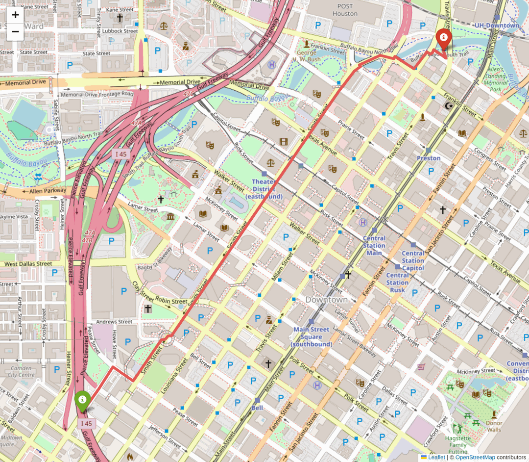
Figure 2: The fastest walking route across downtown Houston, from the green start marker to the red end marker, computed by your RoutePlanner and rendered by draw_route as an interactive folium map. Opening the saved route_map.html lets you pan and zoom it in the browser.
Putting It Together
From six toy towns to a real city, every question maps to the right tool. This table is the capstone in miniature, the mapping from "what is the question" to "which tool answers it":
| The question | The tool | Lesson | Complexity |
|---|---|---|---|
| Is every place reachable? | BFS flood fill | 13 | O(V + E) |
| Fewest stops between two places? | BFS shortest path | 13 | O(V + E) |
| Fastest route between two places? | Dijkstra + min-heap | 20, 9 | O((V + E) log V) |
| Fastest route on a real map? | A* (Dijkstra + heuristic) | 20 | O((V + E) log V), far fewer nodes |
| Cheapest roads to connect everything? | Kruskal's MST + union-find | 20 | O(E log E) |
Bonus: Extend Your Planner
The planner is a real foundation. Each of these upgrades is a small change that pulls in more of the course:
- One-way roads, make
add_roadoptionally directed (append to only one town) to model one-way streets. Reachability and Dijkstra still work unchanged. - Scenic rebates (negative costs), if some roads had negative weights, Dijkstra would break. Swap in Bellman-Ford (Lesson 20), which handles them and even detects negative cycles.
- Cache the map, save the downloaded network with
ox.save_graphml()and reload it offline, so your planner runs instantly without hitting the network every time. - Prim instead of Kruskal, rebuild
cheapest_networkwith Prim's algorithm (Lesson 20) and confirm you get the same total, 33 minutes.